BiCE 2025 Lecture 02
Perceptrons, Artificial Neural Networks and Gradient Descent
Emre Neftci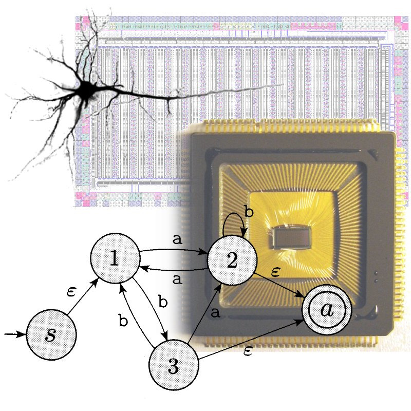
The First Artificial Neuron
-
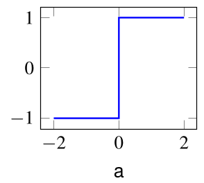
In 1943, Warren McCulloch and Walter Pitts propose first artificial neuron, the Linear Threshold Unit.
$f$ is a step function: $$ y = \begin{cases} f(a) &= 1\text{ if } \ge 0\\ f(a) &= 0\text{ if } a< 0\\ \end{cases} $$
$a$ is a weighted sum of inputs $x$
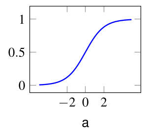
- "Modern" artificial neurons are similar, but $f$ is typically a rectified linear function and variants or $\tanh$

Some Definitions in the Artificial Neuron
- $x_i$ is the output of the pre-synaptic neurons
- $w_i$ is the weight of the connection
- $b$ is a bias
- The total input to the neuron is: $$ a = \sum_i w_i x_i + b $$
- The output of the post-synaptic neuron is: $$ y = f(a) $$
- where $f$ is the activation function
Logic Gates
-
Logic gates are (idealized) devices that perform one logical operation
Common operations are AND, Not, and OR and can perform Boolean logic
Using only Not AND (NAND) gates, any boolean function can be built.

| INPUT | OUTPUT | |
| A | B | A NAND B |
| 0 | 0 | 1 |
| 0 | 1 | 1 |
| 1 | 0 | 1 |
| 1 | 1 | 0 |
Any boolean function can be built out of Mculloch and Pitt Neurons
The Perceptron
- The Perceptron is a special case of the linear threshold unit: $$ y = \begin{cases} -1 & \text{if } a = \sum_j w_j x_j + b \leq 0 \\ 1 & \text{if } a = \sum_j w_j x_j + b > 0 \end{cases} $$
- Three inputs $x_1$, $x_2$, $x_3$ with weights $w_1$, $w_2$, $w_3$, and bias $b$

Perceptron Example
-
Like McCulloch and Pitts neurons, Perceptrons can be hand-constructed to solve simple logical tasks
Let's build a "sprinkler" that activates only if it is dry and sunny.
Let's assume we have a dryness detector $x_0$ and a light detector $x_1$ (two inputs)

| Sunny | Dry | $a$ | $y$ | $t$ |
|---|---|---|---|---|
| 1 (yes) | 1 (yes) | 1 | ||
| 1 (yes) | 0 (no) | 0 | ||
| 0 (no) | 1 (yes) | 0 | ||
| 0 (no) | 0 (no) | 0 |
-
Find $w_0$, $w_1$ and $b$ such that output $y$ matches target $t$
| $w_0 =$ 0 | $w_1 =$ 0 | $b =$ 0 |
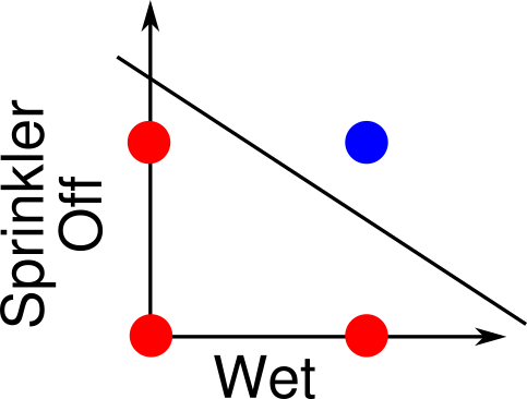
Perceptron Example
- The Sprinkler detects the state "dry" and "sunny": it is like an AND gate.
![]()
- Any boolean function can be built out of Mculloch and Pitt Neurons (=Perceptrons)

Towards Learning: The Perceptron
- Learning parameters $w_i$ and $b$ instead of hand-crafting them Further reading: Professor’s perceptron paved the way for AI – 60 years too soon
The Perceptron Learning Rule
To minimize error, repeat for every misclassified data sample $n$:
$$ w_i \leftarrow w_i + \eta x_{n,i} t_n $$ $$ b \leftarrow b + \eta t_n $$where $\eta$ is called a "learning rate"
- If $y_n = t_n$ no change
- If $t_n = -1$ $\Rightarrow$ $y_n = 1$: subtract inputs $x_{n,i}$ to weights
- If $t_n = 1$ $\Rightarrow$ $y_n = -1$: add inputs $x_{n,i}$ from weights
The Perceptron Learning Rule
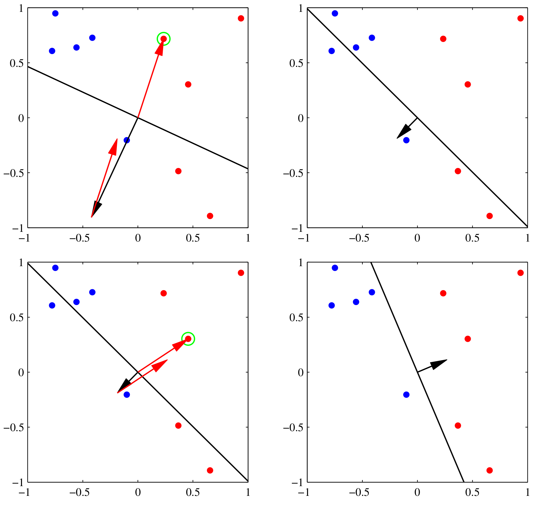
(Bishop, 2006 Pattern Recognition and Machine Learning)
- Perceptron convergence theorem: if the training dataset is linearly separable, then the perceptron learning rule is guaranteed to find an exact solution
(Rosenblatt, 1962, Principles of Neurodynamics: Perceptrons and the Theory of Brain Mechanisms)
Cost Functions
- The Cost (Error) function returns a number representing how well a model performed.
- Perceptrons' cost function is the "Number of Misclassified Samples"
- Other common cost functions are
-
Mean Squared Error: $$ C_\text{MSE} = \frac{1}{2N} \sum_{n \in \text{train}} \sum_k (y_{n,k} - t_{n,k}) ^2 $$
Cross-Entropy: $$ C_{XENT} = - \frac1N \sum_{n \in \text{train}} \sum_k y_{n,k} \log t_{n,k} $$
- The objective in machine learning is to minimize the cost function.
- Cost functions can be minimized using an optimization algorithm
- Cost functions often derive from negative log-likelihood ($- \log p(\mathbf{y}|\mathbf{x}; \theta)$). The cost function depends on the nature of $p$.
Optimization Algorithm: Gradient Descent
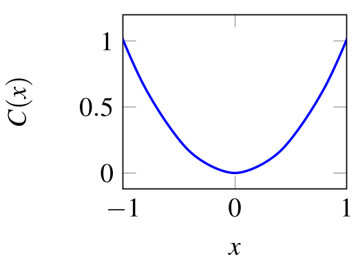
- Example: Find $x$ that minimizes $C(x) = x^2$
- Incremental change in $\Delta x$: $$ \Delta C \approx \underbrace{\frac{\partial C}{\partial x}}_{\text{=Slope of }C(x)} \Delta x $$
- Gradient Descent rule: $\Delta x = - \eta \frac{\partial C}{\partial x}$, $\Delta C \approx - \eta \left( \frac{\partial C}{\partial x} \right)^2$
- Gradient Descent for finding the optimal $x$: $$ x \leftarrow x - \eta \frac{\partial C}{\partial x} $$
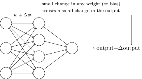
Differentiability and Gradient Descent
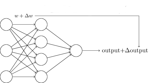
- Derivative of output: $$\frac{\partial y}{\partial w_j} = \frac{\partial f(a)}{\partial w_j} = \underbrace{\frac{\partial f(a)}{\partial a}}_{f'(a)} \frac{\partial a}{\partial w_j}$$
- The function $f'$ needs to be differentiable
- Perceptron's $f$ is non-differentiable: tiny $\Delta w$ can induce a large $\Delta y$
Deriving the Perceptron Rule from Gradient Descent
- The Perceptron criterion is specifically chosen to avoid the discontinuity problem
$$ C_P(\mathbf{w}) = - \sum_{n\in \mathcal{M}} \underbrace{(\sum_k x_{n,k} w_k)}_{a} t_n $$ $\mathcal{M}$ is the set of misclassified samples - Intuition: for misclassified samples $y\cdot t$ will always be negative. $y$ and $a$ have the same sign by definition of the activation function.
- Derivative:
$$ \frac{\partial}{\partial w_i} C_P(\mathbf{w}) = - \sum_{n\in \mathcal{M}} \frac{\partial}{\partial w_i}(\sum_k x_{n,k} w_k) t_n = - \sum_{n \in \mathcal{M}} x_{n,i} t_n $$ -
Parameter Update:
$$ \Delta w_i = -\eta \frac{\partial}{\partial w_i} C_P(\mathbf{w}) = \eta\sum_{n\in \mathcal{M}} x_{n,i} t_n $$
Back to Logic Gates
-
Logic gates are (idealized) devices that perform one logical operation
Common operations are AND, Not, and OR and can perform Boolean logic
Using only Not AND (NAND) gates, any boolean function can be built.
| INPUT | OUTPUT | |
| A | B | A NAND B |
| 0 | 0 | 1 |
| 0 | 1 | 1 |
| 1 | 0 | 1 |
| 1 | 1 | 0 |
Any boolean function can be built out of Mculloch and Pitt Neurons
So we can learn any Boolean function with a Perceptron?
Linear separability
A perceptron is equivalent to a decision boundary.
A straight line can separate blue vs. red
There is no straight line that can separate blue vs. red
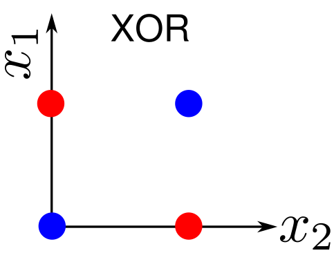
Problems where a straight line can separate two classes are called Linearly Separable
Most complex problems are not linearly separable
Random Projections
What happens if we randomly project the input to a larger space?
Multilayer neural networks can be viewed as targeted projections into a larger space
Neural Network
We can connect Perceptrons together to form a multi-layered network.
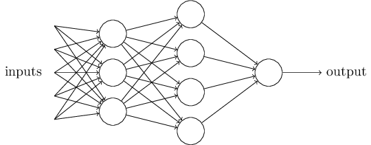
-
If a neuron produces an input, it is called an input neuron
If a neuron's output is used as a prediction, we will call it an output neuron
If a neuron is neither and input or an output neuron, it is a hidden neuron
- Increased level of abstraction from layer to layer
Also called Multilayer Perceptrons or MLP (although units are not always Perceptrons)
Deep neural networks
How many hidden layers and how many units per layer do we need? The answer is at most two
Hertz, et al. 1991

Szegedy et al. 2014
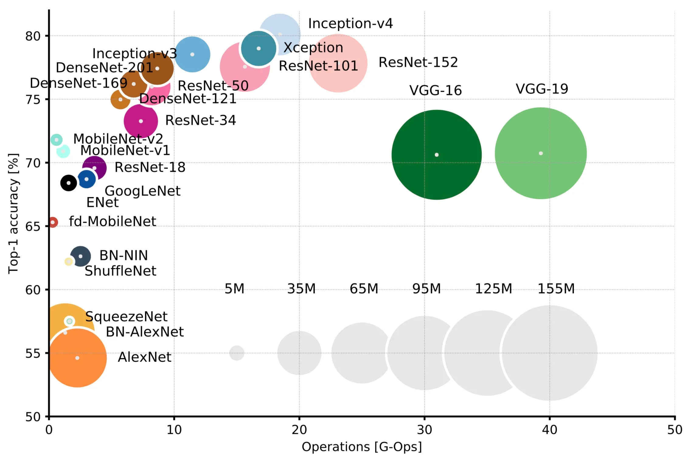
Canziani et al. 2018
Credit Assignment Problem
Credit assignment: which hidden unit weight should we modify to reach a target output?
Continuous Output Neurons (Sigmoid Neuron)
Neurons in deep neural networks are similar to Perceptrons, but with a continuous activation function
Single Layer Network with Sigmoid Units M
- Weight matrix: $W^{(1)} \in \mathbb{R}^{N\times M}$ (meaning $M$ inputs, $N$ outputs) $$ y^{(1)}_i = \sigma(\underbrace{\sum_j W^{(1)}_{ij} x_j}_{a_i^{(1)}}) \\ $$
- Mean Squared Error (MSE) loss function, assuming a single data sample $\mathbf{x}\in\mathbb{R}^{M} $, and target vector $\mathbf{t}\in\mathbb{R}^{N}$ $$ \mathcal{L}_{MSE} = \frac{1}{2} \sum_k(y^{(1)}_k - t_k)^2 $$
- Gradient w.r.t. $W^{(1)}_{ij}$ (in scalar form): $$ \frac{\partial }{\partial W^{(1)}_{ij}} \mathcal{L}_\text{MSE}= (y^{(1)}_i - t_i) \sigma'(a^{(1)}_i) x_j $$
Single Layer Network with Sigmoid Units
Neural networks operations are generally written in vector form
- $\delta^{(1)}$ $\in \mathbb{R}^{N\times 1}$, $\mathbf{x}$ $\in \mathbb{R}^{M\times 1} \leftrightarrow \mathbf{x}^\top$ $\in \mathbb{R}^{1\times M}$. So $\mathbf{\delta}^{(1)} \mathbf{x}^\top$ is an outer product
- $\Delta W \in \mathbb{R}^{N\times M}$: Dimension of $\Delta W$ must be same as $W$!
Two Layer Network with Sigmoid Units
- Two layers means we have two weight matrices $W^{(1)}$ and $W^{(2)}$
- $W^{(1)} \in \mathbb{R}^{N^{(1)}\times M}$, $W^{(2)} \in \mathbb{R}^{N^{(2)}\times N^{(1)}}$
- The output is a composition of two functions: $$ \begin{split} \mathbf{y}^{(1)} &= \sigma(W^{(1)} \mathbf{x} ) \\ \mathbf{y}^{(2)} &= \sigma(W^{(2)} \mathbf{y}^{(1)} ) \\ \end{split} $$
-
Loss function $ \mathcal{L}_{MSE} = \sum_{i=1}^{N^{(2)}}(y^{(2)}_i - t_i)^2 $
Gradient wrt $W^{(2)}_{ij}$ is: $ \frac{\partial }{\partial W^{(2)}_{ij}} \mathcal{L}_\text{MSE}= \underbrace{(y^{(2)}_i - t_i) \sigma'(a^{(2)}_i)}_{\delta^{(2)}_i} y^{(1)}_j $
Gradient wrt $W^{(1)}_{jk}$ is: $ \frac{\partial}{\partial { W_{jk}^{(1)}}} \mathcal{L}_{\text{MSE}} = \underbrace{(\sum_i \delta_i^{(2)} W^{(2)}_{ij}) \sigma'(a^{(1)}_j)}_{\text{backpropagated error}\, \delta^{(1)}_{j}} x_k $
This is a special case of the gradient backpropagation algorithm
The Backpropagation (BP) Algorithm
The task of learning is to minimize a cost function $\mathcal{L}$ over the entire dataset. In a neural network, this can be achieved by gradient descent, which modifies the network parameters $\mathbf{W}$ in the direction opposite to the gradient: $$ W_{ij} \leftarrow W_{ij} - \eta \Delta W_{ij}, \text{where } \Delta W_{ij} = \frac{\partial \mathcal{L}}{\partial W_{ij}} = \frac{\partial \mathcal{L}}{\partial y_i} \frac{\partial y_i} {\partial a_i } \frac{\partial a_i} {\partial W_{ij}} $$ with $a_i = \sum_j W_{ij} x_j$ the total input to the neuron, $y_i$ is the output of neuron $i$, and $\eta$ a small learning rate. The first term is the error of neuron $i$ and the second term reflects the sensitivity of the neuron output to changes in the parameter. In multilayer networks, gradient descent is expressed as the BP of the errors starting from the prediction (output) layer to the inputs. Using superscripts $l=0,...,L$ to denote the layer ($0$ is input, $L$ is output): $$ \begin{split} \frac{\mathrm{\partial}}{\mathrm{\partial} W^{(l)}_{ij}} \mathcal{L} &= \delta_i^{(l)} y^{(l-1)}_j\\ \text{ where }\delta_i^{(l)} &= \sigma'\left(a_i^{(l)} \right) \sum_k \delta_{k}^{(l+1)} W_{ik}^{\top,(l)} \end{split} $$ where $\sigma'$ is the derivative of the activation function, and $\delta_{i}^{(L)}=\frac{\partial \mathcal{L}}{\partial y_i^{(L)}}$ is the error of output neuron $i$ and $y_{i}^{(0)}=x_i$ and $\top$ indicates the transpose.
Common Vector Derivatives
- The expressions above can be written in vector form for a more compact notation.
- A comprehensive resource can be found in (Parr and Howard, 2018), but you must know the following:
$y$ $x$ Scalar Vector Scalar $\frac{\partial y}{\partial x} \in \mathbb{R}^1$ "Derivative" $\frac{\partial \mathbf{y}}{\partial x} \in \mathbb{R}^{N} $ "Vector derivative" Vector $\frac{\partial y}{\partial \mathbf{x}} \in \mathbb{R}^{1\times N}$ $\nabla_\mathbf{x} y \in \mathbb{R}^{N\times 1}$
"Gradient"$\frac{\partial \mathbf{y}}{\partial \mathbf{x}} \in \mathbb{R}^{N\times M}$ Jacobian
Common Vector Derivatives
- Vectors are considered column vectors $ \in \mathbb{R}^{M\times 1}$, Matrices are $\in \mathbb{R}^{N\times M}$
| Scalar | Vector | Matrix | |
| Chain rule | $\frac{\partial f(a(x))}{\partial x} = \frac{\partial f(a(x))}{\partial a} \frac{\partial a}{\partial x} $ | $\frac{\partial \mathbf{f}}{\partial x} = \frac{\partial \mathbf{f}}{\partial \mathbf{a}} \frac{\partial \mathbf{a}}{\partial x} $ | |
| Product | $\frac{\partial ( wx )}{\partial w} = x $ $\frac{\partial ( wx )}{\partial x} = w $ |
$\frac{\partial (\mathbf{w}^\top \mathbf{x})}{\partial \mathbf{x}} = \mathbf{w}^\top$ $\frac{\partial (\mathbf{w}^\top \mathbf{x})}{\partial \mathbf{w}} = \mathbf{x}^\top$ $\frac{\partial (\mathbf{x}^\top \mathbf{x})}{\partial \mathbf{x}} = 2\mathbf{x}^\top$ |
$\frac{\partial (W \mathbf{x})}{\partial \mathbf{x}} = W$ |
Gradient Descent: The Vectorized Way
$$ \frac{\partial \mathcal{L}_{MSE}}{\partial \mathbf{a}} = \frac{\partial \mathcal{L}_{MSE}}{\partial \mathbf{a}} \frac{\partial \mathbf{a}}{\partial W} $$First, compute gradient wrt $\mathbf{a} \in \mathbb{R}^N$ of $\mathcal{L}_{MSE} = \frac12 \mathbf{e}^{\top} \mathbf{e}$, where $\mathbf{e} = (\mathbf{y}-\mathbf{t})$ and $\mathbf{y} = \sigma(\mathbf{a})$
- $\frac{\partial \mathcal{L}_{MSE}}{\partial \mathbf{a}} = \mathbf{e}^\top \frac{\partial \mathbf{e}}{\partial \mathbf{a}}$ (Chain rule)
- $\frac{\partial \mathcal{L}_{MSE}}{\partial \mathbf{a}} = \mathbf{e}^\top \frac{\partial \mathbf{y}}{\partial \mathbf{a}}$ ($t$ not dependent on $a$)
- $\frac{\partial \mathcal{L}_{MSE}}{\partial \mathbf{a}} = \mathbf{e}^\top diag\left(\sigma^\prime (\mathbf{a}) \right) $
- $\frac{\partial \mathcal{L}_{MSE}}{\partial \mathbf{a}} = (\mathbf{e} \odot\sigma^\prime (\mathbf{a}))^\top$ (notation)
- $\frac{\partial \mathcal{L}_{MSE}}{\partial \mathbf{a}} = \delta^{(1)\top}$ (definition of $\delta^{(1)}$)
Gradient Descent: The Vectorized Way, continued
$$ \frac{\partial C_{MSE}}{\partial W} = \delta^{(1)\top} \frac{\partial \mathbf{a}}{\partial W} $$Second, show that $\delta^{(1)\top} \frac{\partial \mathbf{a}}{\partial W} = \delta^{(1)} \mathbf{x}^\top$
- This is more complicated. Naively, the second term results in a 3D tensor $\in \mathbb{R}^{N\times N \times M}$
- One approach is to vectorize ("flatten") $W$ to a matrix $\bar{W} \in \mathbb{R}^{NM \times 1}$.
- Here is it more intuitive to compute elementwise:
-
$$
\frac{\partial a_i}{\partial W_{kl}} = \underbrace{ \delta_{ik} }_{\mathclap{\text{Kronecker Delta}}} x_l
$$
Kronecker delta $\delta_{ik}$ is $1$ if $i=k$, $0$ otherwise.
- $[\delta^{(1)\top} \frac{\partial \mathbf{a}}{\partial \bar{W}}]_{kl} = \sum_i \delta^{(1)}_i \delta_{ik} x_l = \delta^{(1)}_{k}x_l $ which is $[\delta^{(1)} \mathbf{x}^\top]_{kl}$
Neural Networks with PyTorch
- PyTorch is a machine learning framework that facilitates the implementation of Deep Learning
![]()
- Other modern tools such as Tensorflow or JAX have a similar purpose, but PyTorch is the most widespread and easy to use
- Layer today pytorch tutorial (requires Python programming skills and array programming).
Tensor
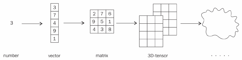
- The tensor is the basic data type of Pytorch (and many other tools likes tensorflow)
![]()
- A tensor is a multi-dimensional array
- For example, a color image could be encoded as a 3D tensor with dimensions of width, height, and color plane.
- Apart from dimensions, a tensor is characterized by the type of its elements (int16, int32, float16, bfloat16, float32, float64, byte, bool etc.).
Tensor Creation
Tensors can be created like numpy arrays
- Numpy
a = np.array([[1,2,3],[3,2,1]])
x = torch.tensor([[1.,2.,3.],[3.,2.,1.]], dtype=torch.float32, device="cpu")
Note float32 is the default for using GPUs (but bfloat16 is increasingly common)
x = torch.tensor(a, dtype=torch.float32, device="cpu") #equivalent
Tensor Types
| IEEE half-precision 16-bit float | ||||||||||||||||||||||||||||||||||
| sign | exponent (5 bit) | fraction (10 bit) | ||||||||||||||||||||||||||||||||
| ┃ |
|
| ||||||||||||||||||||||||||||||||
| 0 | 0 | 1 | 1 | 0 | 0 | 0 | 1 | 0 | 0 | 0 | 0 | 0 | 0 | 0 | 0 | |||||||||||||||||||
| 15 | 14 | 10 | 9 | 0 | ||||||||||||||||||||||||||||||
| bfloat16 | ||||||||||||||||||||||||||||||||||
| sign | exponent (8 bit) | fraction (7 bit) | ||||||||||||||||||||||||||||||||
| ┃ |
|
| ||||||||||||||||||||||||||||||||
| 0 | 0 | 1 | 1 | 1 | 1 | 1 | 0 | 0 | 0 | 1 | 0 | 0 | 0 | 0 | 0 | |||||||||||||||||||
| 15 | 14 | 7 | 6 | 0 | ||||||||||||||||||||||||||||||
| IEEE 754 single-precision 32-bit float | ||||||||||||||||||||||||||||||||||
| sign | exponent (8 bit) | fraction (23 bit) | ||||||||||||||||||||||||||||||||
| ┃ |
|
| ||||||||||||||||||||||||||||||||
| 0 | 0 | 1 | 1 | 1 | 1 | 1 | 0 | 0 | 0 | 1 | 0 | 0 | 0 | 0 | 0 | 0 | 0 | 0 | 0 | 0 | 0 | 0 | 0 | 0 | 0 | 0 | 0 | 0 | 0 | 0 | 0 | |||
| 31 | 30 | 23 | 22 | 0 | ||||||||||||||||||||||||||||||
Tensor Operations
Several operations can be performed on tensors, examples:-
Elementwise Addition
sum_elementwise = x + x # Elementwise addition -
Elementwise Multiplication
product_elementwise = x * x # Elementwise multiplication - Transpose
x_transpose = x.T x.transpose(0,1) #equivalent - Matrix multiplication
          matrix_multiply = torch.matmul(x, x.T) # Matrix multiplication
          matrix_multiply = x @ x.T #equivalent
Graph Representation of an Expression
Pytorch and other frameworks represent a function using a graph (other representations are possible, e.g. a tape)

        v1 = torch.tensor([1.0, 1.0], requires_grad=True)
        v2 = torch.tensor([2.0, 2.0])
        v_sum = v1 + v2
        v_res = (v_sum*2).sum()
Automatic Differentiation
A key feature of machine learning frameworks is automatic differentiation (AD)
- AD cmputes gradients automatically across a set of operations
- Once a backward operation is called on a node, the gradients of all leaf nodes and parameters in the expression are numerically computed
        v_res.backward() #this command computes the gradient
        v1.grad # returns tensor([2., 2.])
v2.grad # returns None
v2.requires_grad #returns False
Neural Network Building Blocks: Modules
Machine learning frameworks can be used for all types of computations, but has predefined modules for constructing neural networks (Linear, Conv, etc.)
- All neural network building blocks are PyTorch modules
torch.nn.Module - Modules are containers for functions, tensors and parameters, can be called like functions
        my_module = torch.nn.Module()
        my_module() #returns NotImplementedError, need to implement this!
        my_module.forward() #equivalent to the previous line
Example: the linear module
- nn.Linear is a class that implements a module
- For example the nn.Linear module defines the linear transformation $$\mathbf{y} = W\mathbf{x} + \mathbf{b}$$
          lin = torch.nn.Linear(in_features = 2, out_features = 5)
          x = torch.tensor([1, 2])
          y = lin(x)
PyTorch Neural Network Building Block: Module
- Modules can be composed to build a neural network. The simplest method is the "sequential" mode that chains the operations
          my_first_nn = torch.nn.Sequential(
                torch.nn.Linear(2, 5),
                torch.nn.Sigmoid(), #this is an activation function
                torch.nn.Linear(5, 20),
                torch.nn.Sigmoid(),
                torch.nn.Linear(20, 2))
my_first_nn(x)
Note that output dimensions of layer $l-1$ must match input dimensions of current layer $l$!
GPUs and Tensors
-
By default, tensors are stored in the CPU (main memory)
b.device
b_cuda = b.cuda(); b_cuda = b.to('cuda') #Both have the same effect
Fully-connected Feedforward Networks (MLP)
- Consists of fuly connected (dense) layer.
- Implements the function: $$ \mathbf{y} = \sigma \left( W \mathbf{x} + \mathbf{b}\right) $$
- $W$ are trainable weights
- $\mathbf{b}$ are trainable biases
- $\sigma$ is an activation function
          linear = torch.nn.Linear(in_features=10, out_features=5)
          x = torch.rand(10)
          y = torch.sigmoid(x)
PyTorch Neural Network Building Block: Module
- Modules can be composed to build a neural network. The simplest method is the "sequential" mode that chains the operations
          my_first_nn = torch.nn.Sequential(
                torch.nn.Linear(2, 5),
                torch.nn.Sigmoid(), #this is an activation function
                torch.nn.Linear(5, 20),
                torch.nn.Sigmoid(),
                torch.nn.Linear(20, 2))
my_first_nn(x)
Note that output dimensions of layer $l-1$ must match input dimensions of current layer $l$!
Activation Functions
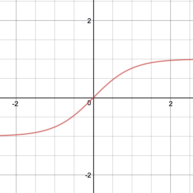
$ \sigma(z) = \frac{1} {1 + e^{-z}} $
torch.sigmoid $ tanh(z) = 2\sigma(z)-1 $
torch.sigmoid $$ y = Relu(a) = \begin{cases} a&\text{ if } a \ge 0\\ 0&\text{ if } a< 0\\ \end{cases} $$
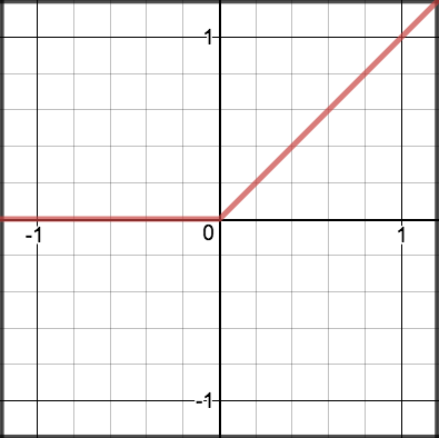
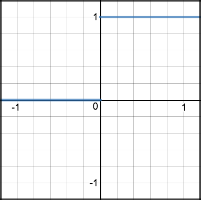
torch.relu $$ y = Step(a) = \begin{cases} 1 &\text{ if } \ge 0\\ 0 &\text{ if } a< 0\\ \end{cases} $$
torch.sign Modern Activation Functions (2024)
$$ y = x\cdot \frac12 \left( 1 + \mathrm{erf}(\frac{x}{\sqrt{2}}\right) $$
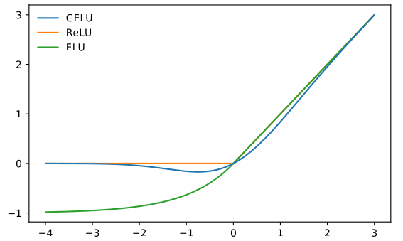
torch.nn.GELU Hendrycks, Dan, and Kevin Gimpel. "Gaussian error linear units (gelus)." arXiv preprint arXiv:1606.08415 (2016)
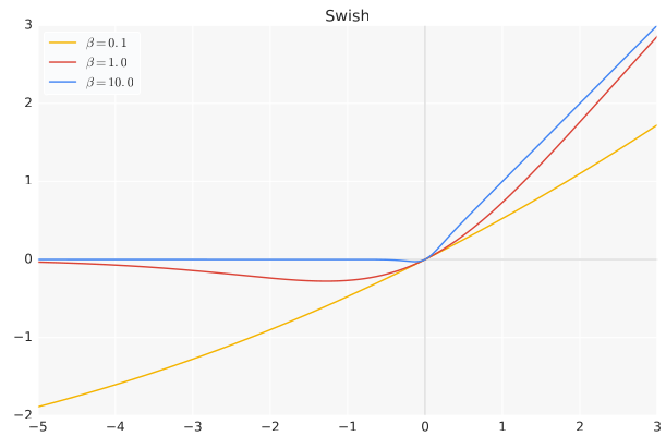
torch.nn.SiLU Ramachandran, Prajit, Barret Zoph, and Quoc V. Le. "Searching for activation functions." arXiv preprint arXiv:1710.05941 (2017).
Loss functions
-
torch.nn.MSELoss: Mean-Squared Error, default for regression tasks
$$ L_{MSE} = \frac{1}{2N} \sum_{n} \sum_i (y_{n,i}-t_{n,i})^2 $$
mse_func = torch.nn.MSELoss() y = torch.tensor([[3.1, 0.9], [-5.1, 2.9]]) t = torch.tensor([[1,0],[0,1]]) loss = mse_func(y, t) -
torch.nn.CrossEntropyLoss: Default for classification tasks
$$L_{XENT} = - \frac1N \sum_n \sum_i t_{n,i} \log y_{n,i}$$
  xent_func = loss = torch.nn.CrossEntropyLoss()
  y = torch.tensor([[3.1, 0.9], [-5.1, 2.9]]) #must be logits
  t = torch.tensor([0,1]) #must be integers
  loss = xent_func(y, t)
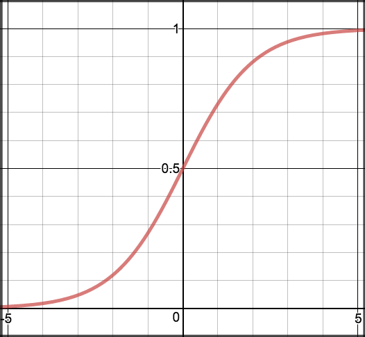
Why Cross Entropy?
- In classification, we are interested in the probability of a category given input $\mathbf{x}$ and prediction $z$:
$$p(z| \mathbf{x}; \Theta)$$
where $z \in \mathbb{N}$
i.e. $p$ is a categorical (multinouilli) distribution (for N classes, a biased N-sided die)
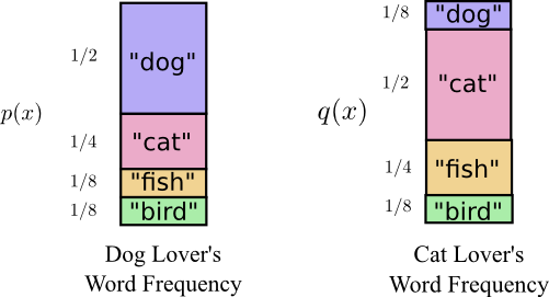
- Class labels $t$ provide ground truth multinomial distribution $$q(t| x)=1$$
- To learn the ground true distribution, we should modify the parameters $\Theta$ such that $p(z|\mathbf{x},\Theta)$ is closer to $q$
- Minimizing a quantity called Cross-entropy $H_p(q)$ is one way to achieve this $$ H_p(q) = -\sum_z q(z)\log_2\left(p(z)\right) $$
Cross Entropy
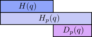
- Cross-entropy (XENT): Average length of a message from $q$ using code for $p$
![]()
![]()
https://colah.github.io/posts/2015-09-Visual-Information/
- The average length of communicating an event from one distribution with the optimal code for another distribution is called the cross-entropy: $H_p(q) = H(q) + D_{KL}(q||p)$
- Minimizing XENT is similar to minimizing the Kullback-Leibler (KL) divergence (noted $D_{KL}$), which is itself a measure of distance between probability distributions.
Cross Entropy Loss
-
For targets with no uncertainty, $q(z|x)=1$ if $z=t$, and $q(z|x)=0$ otherwise.
$$\begin{split}
H_p(q|\mathbf{x}) &= -\sum_z q(z|x)\log_2\left(p(z|\mathbf{x})\right) \\
H_p(q|\mathbf{x}) &= - \log_2\left(p(z=t|\mathbf{x})\right)
\end{split}$$
We define our network output $y_i(x)$ to be the likelihood $p(z=i|\mathbf{x})$, for $i=1,\ldots,N$, where $N$ is the number of categories.
$$\begin{split}
\mathcal{L}_{XENT} &= - \log_2\left(y_{t}(\mathbf{x})\right)
\end{split}$$
But $\sum_i p(z=i|\mathbf{x}_n)= \sum_i y_i(\mathbf{x})$ should sum to one! So far our network does not have such a restriction.
Softmax
- The Softmax function to ensure that the outputs are normalized $$\frac{\exp(a_{n,i})}{\sum_j\exp(a_{n,j})}$$
- Cross entropy becomes
$$\begin{split}
\mathcal{L}_{XENT} &= \log\left(\exp(a_{n,i})\right) - \log\left(\sum_j \exp(a_{n,j})\right)\\
\mathcal{L}_{XENT} &= a_{n,i} - \underbrace{\log(\sum_j \exp}_\text{``Log-Sum-Exp''}(a_{n,j}))
\end{split}$$
-
The exp "undos" the log. Softmax is invariant to an addition of a constant
Use the softmax only when the loss involves a log function! Don't use it with MSE!
Loss functions and optimizers
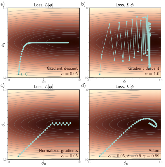
- The loss/fitness function defines our objective. An optimizer defines the strategy to minimize/maximize the loss function.
- Common gradient-based optimizers:
- SGD : A vanilla stochastic gradient descent algorithm
- RMSprop : An optimizer that normalizes the gradients using moving root-mean-square averages
- Adam : An adaptive gradients optimizer (de facto optimizer in DL)
The Training Loop
All the parts of the machine learning algorithm come together in the training loop, i.e. proceeding iteratively over data samples and make gradient updates.
- Create a neural network, cost function and optimizer
- In a loop:
- Compute the neural network loss
- Take the gradient of the loss using .backward()
- Run one optimization step (= apply the gradient)
def train_step(data, tgt, net, opt_fn, loss_fn):
    y = net(data)
    loss = loss_fn(y, tgt)
    loss.backward()
    opt_fn.step()
    opt_fn.zero_grad()
    return loss
for i in range(100):
    print(train_step(b, t, my_first_nn, opt, mse_loss))
Universal Approximation Theorem
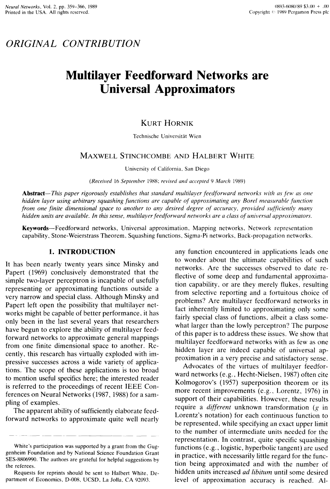
A feedforward network with a linear output layer and at least one hidden layer with any “squashing” activation function (e.g. Sigmoid) can approximate any Borel measurable function (any continuous function on a closed and bounded subset of $\mathbb{R}^n$) with any desired nonzero amount of error, provided that the network is given enough hidden units.
Why does Machine Learning Work?
How can we affect performance on the test set when we can observe only the training set?The field of statistical learning theory provides some answers.
Generalization error
In ML, the objective is generally to perform well on new, previously unseen inputs. The ability to perform well on new inputs is called generalization.
- We train on the training set but we care mainly about the test set $\mathcal{D}_{test}$, for example minimizing the value of $$ \mathcal{L}_{MSE}(\mathcal{D}_{test};\Theta) = \frac{1}{N_{test}} (f(X_{test};\Theta) - \mathbf{y}_{test})^2 $$
- A central assumption here is that the training samples are "representative" of the test samples, in other words we require the two sets to be independent and identically distributed (iid).
- The distribution generating the train and test sets is called the data-generating distribution
- It is crucial to never use the test samples (also called test split) during training.
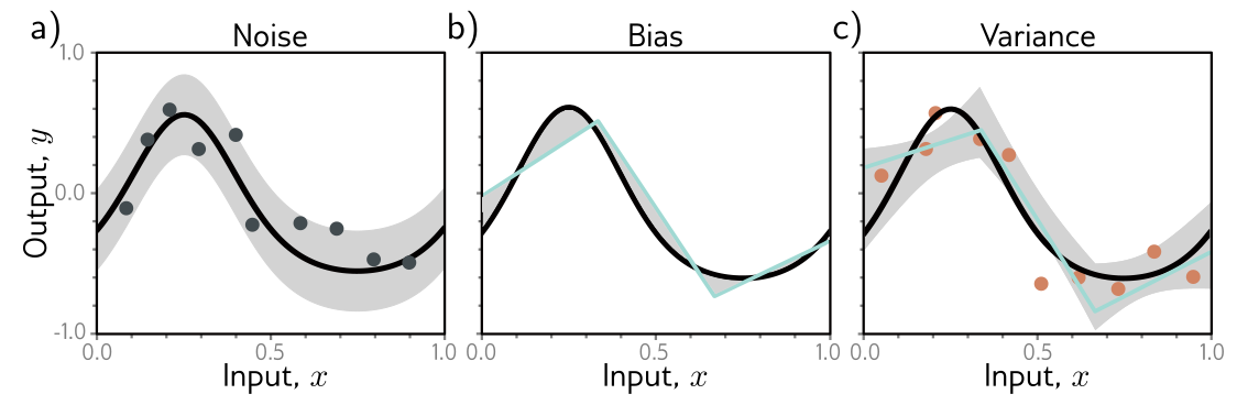
Sources of Error: Noise, Bias, and Variance
Understanding Deep Learning, Prince 2023 [Chap.8]
- Noise: Data generation is noisy
- Bias: Model is not flecible enough
- Variance: The model training is not perfect, e.g. limited training samples
All three sources contribute to the test error
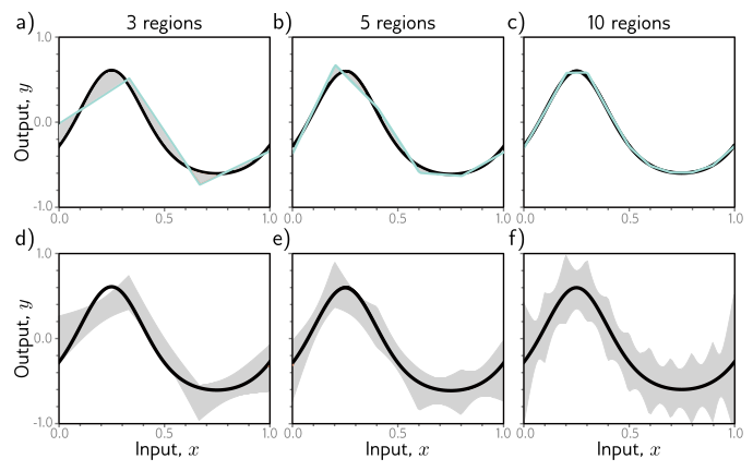
Bias-Variance Trade-off
Increasing the model capacity does not necessarily reduce the test error. This is known as the bias-variance trade-off.
Understanding Deep Learning, Prince 2023 [Chap.8]
$$ L[x] = \bigl(\text{f}[x,\boldsymbol\phi]-y[x]\bigr)^2 $$ $$ \mathbb{E}_{\mathcal{D}}\Bigl[\mathbb{E}_{y}[L[x]]\Bigr] = \underbrace{\color{black}\mathbb{E}_\mathcal{D}\Bigl[\bigl(\text{f}[x,\boldsymbol\phi[\mathcal{D}]]- \text{f}_{\mu}[x]\bigr)^2\Bigr]}_{\text{variance}} + \underbrace{\color{black}\bigl(\text{f}_{\mu}[x]\!-\!\mu[x]\bigr)^2}_{\text{bias}} + \underbrace{\color{black}\sigma^2}_{\text{noise}} $$
Underfitting and Overfitting
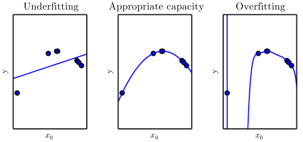
Understanding Deep Learning, Prince 2023 [Chap.8]
- The factors determining the performance of an ML algorithm are
- Small training error (prevent underfitting)
- Small gap between training error and test error (prevent overfitting)
Double Descent
Test error decreases again in the over-parameterized regime (= more parameters than data points) - count er to the bias--variance trade-off
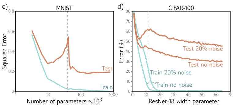
The first part of the curve is referred to as the classical or under-parameterized regime, and the second part as over-parameterized regime.
Double descent is not fully understood, but foundation models (e.g. GPT-3) are trained in the over-parameterized regime.
Further Reading and Bibliography
- Understanding Deep Learning Simon Prince, 2023
- Perceptron Introduction from (Bishop et al. 2006) Chapter 4
- Most material from (Goodfellow et al. 2016), chapters 5 and 6
- Gradient calculus for neural networks (Parr and Howard, 2018)